
School Bus Route Optimization: A GIS and Operations Research Approach
How to approach school bus route optimization using GIS and operations research: Marion County baseline metrics, synthetic route diagrams, scenario economics, stop/ride-time trade-offs, safety constraints, and equity analysis.
School districts across the country operate bus fleets that cover millions of miles annually. Most route planning still happens through incremental manual adjustments rather than systematic optimization. The gap between current practice and what modern GIS and operations research can deliver is substantial.
This article walks through the methodology for a route-optimization feasibility study, using Marion County Public Schools in Florida as a reference case. The principles apply to any district with staggered bell times, diverse geography, and enough scale to justify the analysis.
Data note: Figures below use publicly available district and state sources. Route diagrams are synthetic examples, not real student locations. No student-specific transportation data is used.
Why Marion County is a strong optimization candidate
Marion County operates hundreds of buses across a large, geographically mixed county, with more than six million annual route miles. At that scale, even modest improvements in stop placement, route sequencing, and schedule reliability can produce meaningful operational gains.
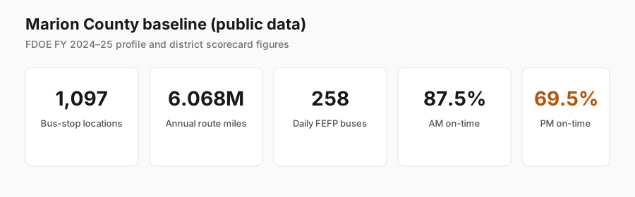
| Baseline metric | Value | Optimization implication |
|---|---|---|
| Bus-stop locations | 1,097 | Large candidate set for safe consolidation and redesign |
| Annual regular route miles | 6,068,000 | Single-digit percentage reductions matter systemwide |
| Daily FEFP buses | 258 | Fleet chaining and tiering are important |
| Eligible students transported | 19,631 | Demand is large enough for joint stop-and-route modeling |
| AM on-time | 87.5% | Morning service appears relatively more stable |
| PM on-time | 69.5% | Afternoon reliability is a prime optimization target |
| Transportation operating expenditures | ~$28.08M | Scale supports a controlled pilot with measurable ROI |
The reliability gap is especially important. Optimization should focus not only on miles, but also on traffic variability and pickup-time robustness. The district already staggers school start times: most elementary schools at 7:35 AM, high schools at 8:30 AM, middle schools at 9:20 AM. That creates trip-chaining opportunities if route geometry and travel-time buffers actually fit those windows.
What public data can and cannot tell you
A feasibility study can establish the business case using publicly available information:
Available from state education departments:
- Enrollment and transported student counts
- Bus inventory and daily service counts
- Annual route miles and operating expenditures
- Stop location counts (aggregate, not individual addresses)
Available from county GIS:
- School attendance boundaries
- Parcel data with residential classification
- Road networks with attributes
Available from census and DOT:
- School-age population by block group
- Traffic counts and signal locations
- Road safety characteristics
Not available publicly:
- Individual stop locations and sequences
- Student-to-stop assignments
- Actual route geometries
- GPS/AVL history
- Exact ride times and stop-level on-time performance
This distinction matters. Public data can quantify the scale of opportunity. It cannot responsibly recommend moving a specific stop from one street corner to another. That requires the district's internal transportation data.
Building a demand model without student addresses
When actual student addresses are unavailable, you can construct a privacy-preserving demand surface:
- Start with residential parcels from county GIS
- Weight by school-age population share from census block groups
- Clip to school attendance boundaries
- Normalize to match official transported student counts
The result is a set of demand centroids that approximate where students live without using any individual information. This is sufficient for planning-level analysis and pilot scoping.
The optimization problem is multiobjective
School bus routing is not a standard vehicle routing problem. A useful model balances safety, walking burden, student ride time, vehicle capacity, school arrival windows, route miles, driver schedules, and late-arrival risk.
Minimize:
α(Buses Required) + β(Route Miles) + γ(Student Ride Time)
+ δ(Expected Late Minutes) + ε(Student Walking Time)
+ ζ(Safety / Equity Penalties)

Subject to capacity, school time windows, accessibility,
hazardous-walking constraints, and safe boarding/crossing rules.
Those decisions are coupled:
Stop selection: Which candidate locations should be active stops?
Student assignment: Which students use which stops?
Route sequencing: In what order does each bus visit its stops?
Trip scheduling: Which bus serves which school, and can trips be chained across bell tiers?
Research shows that solving these jointly outperforms sequential approaches where stop locations are fixed before routing begins.
Pickup-location optimization
Closely spaced stops may be candidates for consolidation, but distance alone is not enough. A production optimizer should require approved pedestrian access and safe boarding conditions, while treating hazardous road crossings and accessibility requirements as hard constraints.
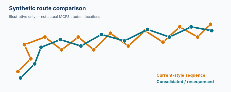
Illustrative only. Current-style sequence vs consolidated/resequenced path. Not actual MCPS student locations.
Florida law makes safety the primary requirement in school bus routing. An optimizer should never trade a hazardous walking path for a shorter route. Candidate stops should be filtered using traffic counts and speeds, crossing characteristics, sidewalk availability, and bus stopping/maneuvering feasibility before optimization, not penalized with a soft cost coefficient after the fact.
Synthetic Ocala experiment
To illustrate the trade-offs, a deterministic example used 64 modeled riders and 22 stops, then consolidated compatible demand and resequenced the route:
| Metric | Current | Optimized | Change |
|---|---|---|---|
| Stops | 22 | 19 | −13.6% |
| Route length | 22.30 mi | 21.72 mi | −2.6% |
| Route duration | 70.02 min | 66.38 min | −5.2% |
| Mean ride time | 37.80 min | 34.68 min | −8.3% |
| Maximum ride time | 70.02 min | 66.38 min | −5.2% |
| Average walk to stop | 0.050 mi | 0.098 mi | +95.5% |
| Maximum walk to stop | 0.159 mi | 0.330 mi | +107.3% |
The key lesson: bus efficiency can improve while walking burden gets worse. That is why a real deployment should use strict grade-level walking limits, accessibility rules, and safe pedestrian-network checks before approving a change.
Pickup-time optimization
Pickup times should be based on historical GPS travel-time distributions rather than one static average speed. For each stop, the schedule can be back-calculated from the school arrival target:
PickupTime(stop i)
= SchoolArrivalTarget
− PercentileTravelTime(i → school)
− ExpectedDownstreamDwell
− ReliabilityBuffer
Because morning and afternoon reliability differ, AM and PM travel-time models should be trained separately. When you consolidate two stops into one, every downstream pickup time on that route changes. The optimization should recalculate the entire trip schedule rather than manually adjust individual times.
What reasonable targets look like
For a district the size of Marion County, planning scenarios can be framed as:
| Scenario | Mileage reduction | Annual route miles avoided | Blended cost exposure |
|---|---|---|---|
| Conservative | 3% | 182,040 | ≈ $0.81M |
| Planning target | 5% | 303,400 | ≈ $1.35M |
| Stretch | 8% | 485,440 | ≈ $2.16M |
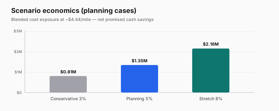
The blended rate of roughly $4.44 per reported mile comes from dividing systemwide transportation operating expenditures by total school-bus miles. That is an accounting ratio, not marginal savings. Fuel and maintenance scale with miles. Labor savings require reducing paid hours, not just shortening routes within existing shifts. Fleet savings require actually removing buses from service.
The honest framing is "cost-equivalent exposure to be validated," not "guaranteed savings."
A useful pilot KPI contract might include:
| Metric | Pilot target |
|---|---|
| Route miles | 5-10% reduction |
| Active stops | 8-15% consolidation where safety permits |
| Mean ride time | 5-8% reduction |
| Deadhead miles | 10%+ reduction |
| Capacity | Zero standees |
| Equity | No subgroup absorbs disproportionate walk/ride burden |
Equity as a constraint, not an afterthought
A cost-only optimizer will systematically favor consolidation in dense neighborhoods even if those areas have weaker pedestrian infrastructure, fewer vehicles per household, or younger students. The model should evaluate changes at the census block group or attendance zone level.
Useful equity metrics include:
- Walking distance change by neighborhood income/demographics
- Ride time change by geography
- Share of students whose stop moves beyond a threshold
- Pickup time shift distribution
- Unsafe crossing exposure
The before/after analysis should confirm that no subgroup absorbs disproportionate burden solely to create districtwide savings.
Production architecture
| Layer | Purpose |
|---|---|
| Transportation data mart | Join anonymized rider assignments, stops, routes, buses, capacities, bell times, GPS pings, and actual arrivals |
| Safety-aware GIS network | Model sidewalks, crossings, speed environments, restricted turns, and approved stop candidates |
| Student-to-stop optimizer | Assign riders to safe stops within grade-appropriate walk limits |
| Vehicle-routing optimizer | Sequence stops, assign buses, and chain trips across school tiers |
| Travel-time model | Learn time-of-day distributions from GPS history |
| Scenario simulator | Compare reliability-first, balanced, and efficiency-first alternatives |
This is not a spreadsheet project. It requires GIS processing, optimization engines, data pipelines, visualization, and export back into district scheduling systems.
Implementation sequence
- Audit route, stop, rider, capacity, GPS, and bell-time data
- Build a safety-aware pedestrian and bus road network
- Generate multiple stop, route, and pickup-time scenarios
- Run explicit safety, accessibility, and equity audits
- Pilot one Ocala urban zone and one rural zone
- Compare GPS actuals against the old schedule, then scale successful changes
A matched A/B design (optimize one route, leave a comparable route unchanged, compare outcomes) provides much stronger evidence than comparing an optimized week against an arbitrary annual average.
Bottom line
Marion County's network is large enough, and its reported afternoon reliability gap significant enough, to justify a modern route-optimization program. The strongest near-term move is to join route schedules with GPS actuals, then use that dataset to improve pickup times and route reliability before attempting aggressive stop consolidation.
Exact street-level recommendations should wait for a secure stop/ridership/AVL extract. Public-data analysis can establish the business case. Measured pilots should decide what scales.
If you operate a school district, transit agency, or logistics fleet and want to explore what GIS and operations research can do for your routing, contact us for a technical conversation.